Understanding XgBoost, A Simple Approach

What is already very clearly established is how effective XgBoost has been, Kaggle winning submissions stand testimony to it. That and the fact that it has neat Parallelization capabilities makes it strong to stack up against, but what has not been as clearly established is its complete understanding. Disclaimer, in no way, do I guarantee that this blog can provide that completeness, but it is a step in that direction. My trouble in learning was online blogs and paper breakdowns were either too vague or too complex, I am going for the just-right spot here.

1.1 Boosting and Bagging

NOTE: Before we start, there are heterogenous and homogenous ensembles, let’s not go down there just yet. Stick to the script and we will be fine.

Lets set the base for what is to come. Assuming you are aware of the term ensemble (if not you know what to do), bagging or Bootstrap Aggregation is simply put, training on the same set of learners but on different data.

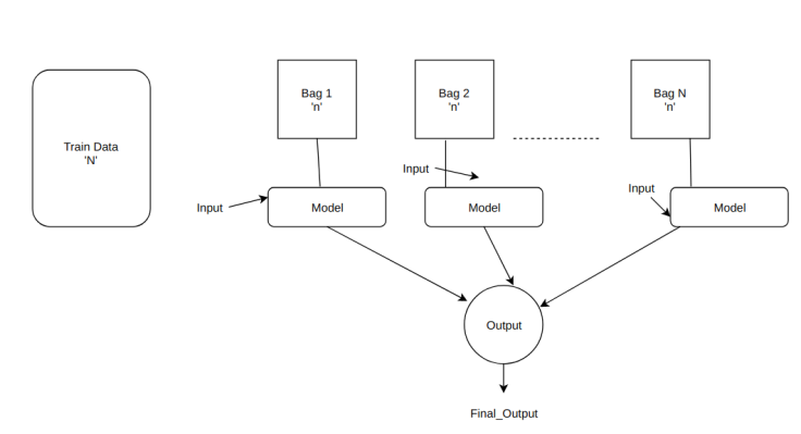
To put more perspective into that, Given we have a dataset with ‘N’ inputs, bagging essentially means ‘v’ bags obtain ‘n’ inputs/ datapoints of its own. How are the datapoints chosen? To be exact they are chosen at random with replacement. With replacement being the caveat here, meaning there can be the same data points in multiple bags. What we see further down below, the ‘Model’ is the learning algorithm. Notice how even though every bag has essentially different data, the Model is the same. Thus for a given input passing it over all these trained models, in theory, should give us better results, as every model is learning from different data, ie different perspectives to be learned upon. Once we have these outputs, a simple vote or mean based on the type of problem is chosen. What aggregates to the final_output is what a wrapped API of a bagging model would throw out at us.

Understanding bagging helps appreciate boosting much better. A question we can ask ourselves at the moment is,

Instead of a random subset everytime why not promote data that requires to be learnt better?

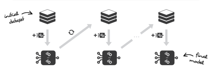
That is exactly what boosting addresses. It starts with the initial data ‘n’, but given it has wrongly classified given set of points from the train set, then the probability of those points occurring in the next bag is increased, this process is chained until the last bag. The goal is we have a better-learned model by the end. (Ada Boost–> Stumps)

1.2 Understanding Decision Trees

Given Decision trees are the fundamental blocks of the XgBoost algorithm, it doesn’t make much sense to go ahead without a clear understanding of Decision Trees first. What are they? Are they just glorified If-Else statements? How do they fit into the larger picture?

Given we have two axes, x1 and x2, our objective is to make cuts such that we can distinctly segregate data. Note, Decision trees are binary trees that seek to do the above and optimize the error/ Loss afterward.

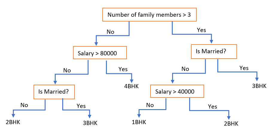
Inhibited only by my lack of talent in drawing, I’ll try to go over a cliche Decision tree that google’s search results came up with. So important takeaways being, features reused at different stages for instance (Is married?) or the fact that the leaf nodes are our classes to be segregated. So are they really just a glorified IF-Else statement? Either way, they are great at what they seek to achieve and are set as base learners/ weak learners in many an ensemble. Something important to takeaway here is that a weak learner is tuned to be a strong learner, in the end, that’s what ensembles really are.

2.1 Breaking down the tree Jargon

In my learning, what I often see is that in Machine Learning in general, once the jargon is broken down, learning the underlying concept becomes very simple. So this next part is all about understanding to speak “Trees”.

Pruning: It is a technique in machine learning and search algorithms that reduces the size of decision trees by removing sections of the tree that provide little power to classify instances. For example in the above classification what if one of the leaf nodes end with zero classified results, aren’t they simply attributing to an unnecessary cut?

Entropy: “The Degree of Randomness”. Simply put in each of these classified leaf nodes, how much is the degree of disorder. Obviously the lesser the better, in other words, lesser the entropy, purer the node is. A common expression of entropy is,

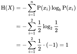
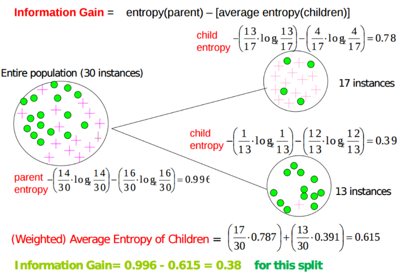
For example, in the child nodes shown, one has more impurity, ie, more entropy, since there is larger variance or different instances. In the second case, the entropy is lesser as the sample node is purer, ie there is a clean line of segregation.

Random Forests: As far as real-world naming conventions go, this one does it best. It is exactly what it is named. A bunch of Decision Trees!

Gradient Boosting: The concept is very close to Boosting/ AdaBoosting that we discussed before. The difference lies in what it does with the under fitted values of its predecessor. Contrary to AdaBoost, which tweaks the instance weights at every interaction, this method tries to fit the new predictor to the residual errors made by the previous predictor and builds on and so forth until maximum estimators are reached or the error function hasn’t changed. Long note short, In theory, a gradient boosted tree kicks Random Forests behind, BigTime! This post by Prince[7] has an amazing step level plot data that helps understand the learning. A numerical understanding of the same is found below in section 2.3.

2.2 What is Regularization?

A useful Link: Regularization-Quora, What follows is an excerpt from the link, that I believe makes most headway in understanding the term.

For any machine learning problem, essentially, you can break your data points into two components — pattern + stochastic noise.

For instance, if you were to model the price of an apartment, you know that the price depends on the area of the apartment, no. of bedrooms, etc. So those factors contribute to the pattern — more bedrooms would typically lead to higher prices. However, all apartments with the same area and no. of bedrooms do not have the exact same price. The variation in price is noise.

Now the goal of machine learning is to model the pattern and ignore the noise. Anytime an algorithm is trying to fit the noise in addition to the pattern, it is overfitting.

And Regularization, simply put is a way to reduce overfitting by artificially penalizing higher degree polynomials and ensuring the model learns only on data, not noise.

2.3 How do Weak learners learn

Understanding this helps us appreciate boosting and its enormous influence in modern-day Machine learning. Analytics Vidhya [6], brings context behind boosting in this post (attached below). I’ll try to do justice to the depiction.

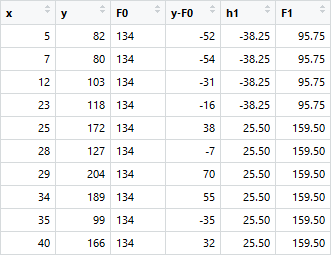
Given the data on years and target variable salary, let’s understand how weak learners from the boosting method make the decisive cuts.

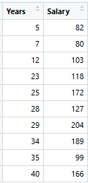
An initial model F0 is defined to predict the target variable y. Let’s start at a fixed value cut for F0. Given that value is 134,

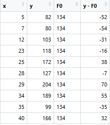
Then we take the loss to be (y-F0) and further cuts are made on the same. For instance, we take x<=23 to be one split and values greater than the later to be another. The node value -38.25 and 25.5 is representative of the mean of the values of x that are below or equal to 23 and the vice-versa.

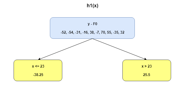
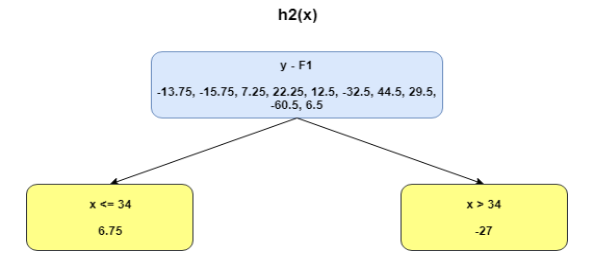
Now the table will shift around new values that are shaped around h1(Shown in Figure). The boosted function F1(x) is obtained by summing F0(x) and h1(x). This way h1(x) learns from the residuals of F0(x) and suppresses it in F1(x). Boosted learner h2 is now (y-F2) and so on until maximum level of optimization [or restricted level based on user parameter option for depth]. Repeating the same over multiple iterations gives me h2, h3, etc. Each time the intuition is that the model picked up errors from the residues and has become slightly better. The MSE below helps appreciate that fact.

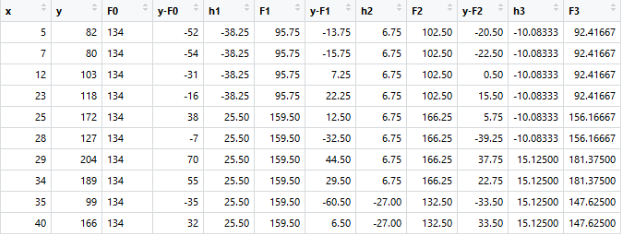
The MSEs for F0(x), F1(x) and F2(x) are 875, 692 and 540. Putting it into perspective the level of improvement for something as simple as a decision tree is staggering.

2.4 Gradient motivated learning, understanding what it means to weight a node

Instead of fitting h(x) on the residuals, fitting it on the gradient of loss function, or the step along which loss occurs, would make this process generic and applicable across all loss functions.

Given we have understood what that means [Gradient is a way to indicate which direction to proceed with], the next logical step is to understand how to define that gradient value.

The following steps are involved in gradient boosting:

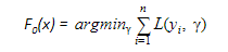
F0(x) – with which we initialize the boosting algorithm – is to be defined:

The gradient of the loss function is computed iteratively:

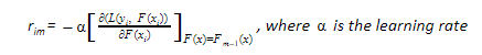
Each hm(x) is fit on the gradient obtained at each step.

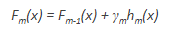
To fully understand the concept of weights on the leaf node, we need to understand how the final boosted model Fm(x) is fit. There exists a multiplicative factor γm, which is weighted with the hm(x), thus the expression would be,

3.1 Please get to XgBoost!

Well enough said about what builds up to XgBoost, but ironically we have already gained a fair understanding of XgBoost. XGBoost (GitHub) is simply one of the most popular and efficient implementations of the Gradient Boosted Trees algorithm, a supervised learning method that is based on function approximation by optimizing specific loss functions as well as applying several regularization techniques.

Lets back up a bit and understand it completely. There are two approaches mentioned in the XgBoost paper.

3.1.1 Exact Greedy Algorithm [1]

Start with a single root (contains all the training examples)
Iterate over all features and values per feature, and evaluate each possible split loss reduction:

gain = loss(father instances) – (loss(left branch)+loss(right branch))
The gain for the best split must be positive (and > min_split_gain parameter), otherwise we must stop growing the branch.